March 25, 2015: Centripetal Acceleration vs Angular Frequency

Objective:

Understand centripetal acceleration and angular frequency, and their relationship.

Set-up:

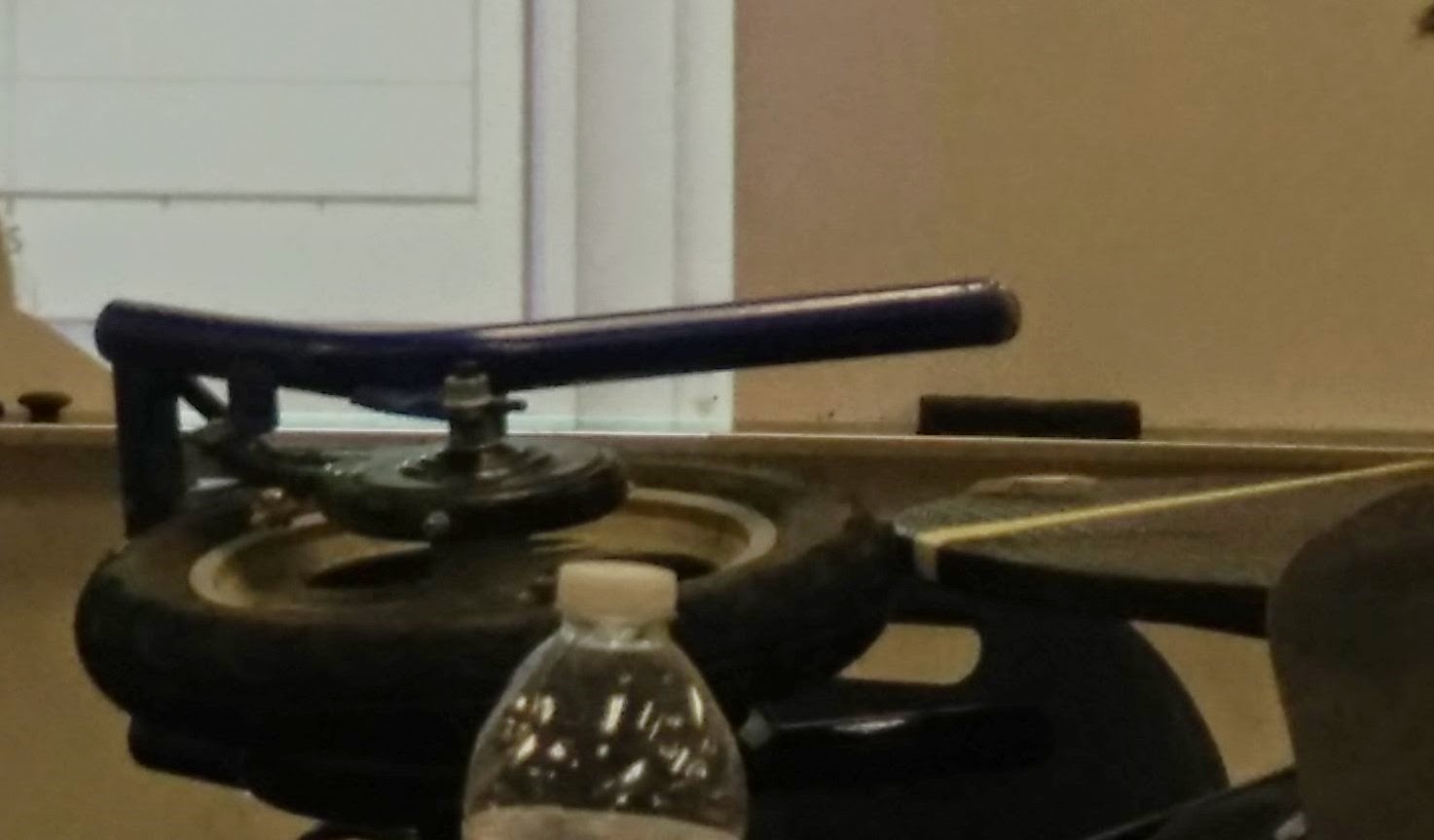
Professor Wolf set up and electric scooter and wheel on a table, and allowed the wheel to be in contact with a metal wheel that could spin. Attached to the metal wheel, was a wireless accelerometer that was linked to a computer where he was going to record the data. Attached to the right (out of view) was a piece of paper and a photogate to measure when the piece of tape went by, therefore completing a revolution.

Experiment:

The professor ran 5 experiments with different voltage, meaning that these would differ in velocity tangent to the electrically operated wheel. The data was then collected along with the time it took to complete 10 rotations. Then He used logger pro to give us a value for acceleration. 

Analysis:

We took the recorded data and used logger pro to try and find a relationship between the centripetal acceleration and the angular frequency omega. We then proceeded to graph an omega squared vs acceleration graph to find their relationship. In our data set "Y" is our acceleration whereas "W^2" is omega squared.

Then we obtained the following graph. We found that our slope in this graph is our radius. it comes in at .1381 meters or 13.81 cm. Which is well within our range.

Summary:

This lab allowed us to visually see the relationship between angular velocity and centripetal acceleration. We saw how the equations we learned where probably found and how they relate to each other. Although our radius was not exact, it did fit within our margin of error. This is to be expected as we had some errors in measurement since the accelerometer might have been slightly off-centered and there might be inconsistency within both wheels structures. However, we were able to find the relationship that {acceleration = radius * omegasquared }.

March 16, 2015: Modeling Friction Forces

Purpose:
The purpose of this lab is to get a better understanding of static friction and kinetic friction. Thru experiment we hope to come up with a model to be able to predict values of acceleration.

Set-up:

Water was added and weighed

Here are all the blocks we used and the balance we used

We weighed each block

We set up our mass on the table, and hanging of the ledge our cup with water

Static Friction:

We took a block and tied string to it and let a cup with water hang on one side, water was added until it the blocks began moving as this would indicate our maximum static friction. The same block was always used in the same position on the bottom to ensure the most accuracy with measuring static friction.

The values we obtained for the masses of the blocks and the required mass to make them move is the following:

We then took the values of normal force and graphed them against a static force required to move them. The using a linear fit we obtained a line with the slope of the coefficient of the static friction.

Kinetic Friction:

For this part of the lab we changed the set-up instead of having the block pulled by water, we connected a force sensor to the string and pulled the sensor (and therefore moving the block) at a constant velocity. We did this 4 times and recorded the data. This data was then analyzed and the mean for each of them was found.

The means were graphed along side the force applied to each of these and the following graph was obtained with the coefficient of static friction being 0.2482 .

Static Friction at a sloped surface:

 We set up the block on a ramp and elevated it until the point were it just started to slide.

In our case, we found the angle of static friction to be 12.7 degrees. Then we drew up a free-body-diagram and solved for the static friction. As we can see here, items just canceled out leaving us with a static coefficient on this surface of 0.325 .

Kinetic friction of downhill block:

We used the same setup a the previous one except we hooked up a motion sensor to the top and increased the angle to ensure a downward acceleration. We choose 22.3 degrees and took measurements of our block sliding down the ramp. What we got was the following data set: 

Our value for acceleration as seen here is of a= 0.320(m/s^2). Since we already knew the mass of our block, again we used newtons laws and solved for our kinetic friction:

As we see here, our final value for our kinetic friction was 0.3745 . 

Prediction the Acceleration:

For this experiment we had to use what we knew about this block in order to predict what would happen if a force where to be applied to it. So we set up a scenario, this included a frictionless pulley and a mass. We knew that a mass of at lease .047kg is required to move our block so we used a 0.74kg mass. 

The following formula was derived for our prediction:

The actual values we got where:

Conclusion:

What we learned in this lab is that static friction is higher than kinetic friction. Once an object starts moving, it takes less force to keep it in motion. We also learned that different surfaces have different friction coefficients, not all materials are the same and have different surfaces. Of course we also had measurement error, but what we saw if fundamentally this: Static friction is higher than kinetic friction.

March 11, 2015: Air Risistance

Purpose:
The Purpose of this lab was to find out how air resistance behaved with falling objects and how this led to the objects having a terminal velocity. In other words, the relationship between air resistance  and the speed of falling objects (in our lab, coffee filters).

Set-up:
The stage for this experiment was the technology building, also know as building 13. The reason for the selection of this building and not just any other place is because the building has this balcony indoors where there are no air currents. This allows us to have a better chance to only deal with vertical air resistance.

Photo taken from balcony where coffee filters were dropped to to the ground
The laptops that were going to record the fall are seen on the stairs.

For this experiment we measured the glass part of the balcony at 1.5m and put this into the scale for our video recording. We dropped air filters from the top and recorded their path to the bottom. On the first run we used only one filter, the next run we added another filter and saw it glide down and proceeded to add one and repeat for 5 times. We then returned to class and began to analyze the videos on logger pro.

We analyzed each video and plotted points to obtain a graph of each acceleration like this one:

Once we had the terminal velocity of each round of coffee filters, we proceeded to obtain the mass of the air filters. Our classmates did the calculations and obtained the value of one coffee filter to be 0.000926Kg. With the information now being sufficient we went off to find a mathematical model to simulate what we had seen. It turns out the equation F= K * (V^n) is our equation for air resistance and K is simply a sensitive value for surface area in contact with the air on the bottom. Once we graphed the combined known values of mass and terminal velocities and created a exponential graph fit we obtained the following graph:

The computer then gave us a value, but just to be sure we used Excel to analyze our data and also calculate our value of air resistance. Using Newtons second law of F=ma we came to the conclution that a=g[(K*V^n)/m]

As we see here, when our acceleration is about 0, our velocity is 1.8867m/(s^2). With a percentage error ~+or - 1%.

Conclusion:

We were able to get a good idea of what air resistance is. In essence it is when the force of the air is the same as the mass of the object falling, thus rendering the acceleration equal to zero. Although we could not completely prove this thru our lab because of uncertainty in the lab equipment, we know this to be true as we came really close. 

March 9, 2015: Propagated Uncertainty in Measurement

Purpose:

The purpose of this lab was to make us understand that there is always uncertainty in every measurement even when using extremely accurate measurement tools. With this in mind, this lab is also designed to help us understand how to calculate this uncertainty into out measurements to be able to compensate for it.

First Procedure:
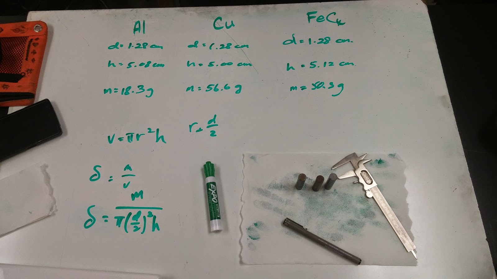
1. We were where given calipers to measure the seize of 3 different metallic cylinders. These were copper, aluminium, and steel.
2. These measurements were recorded

Steel left, Copper center, Aluminum right.  Calipers are to the far right. Measurements were written here for easy viewing.

3. We learned to take partial derivatives since they tell us the uncertainty in our measurements.

4. To do partial integration, we basically make n number of equations and add them together, when n is the number of variables in an equation. 

5. We then then treat each of these individually and take only the derivative of each. When doing this, we treat one as a variable and the rest as a constant.

6. Then when we had the final uncertainty, we plugged in out values to obtain the uncertainty in our measurements.

7. The values we got where the following:

8. The uncertainty for our densities where:

Aluminum was off by + or - 0.2390g/cm
Copper was off by + or - 0.24885g/cm
Steel was off by + or - 0.2372g/cm

Part 2:

For this part we used setup #1 and #2

Setup 1

Setup 2

First we measured the setups and found that setup 1 had the cable on the left being pulled at an angle north of west at 26 degrees with a force of 10.7N. The cable on the right was being pulled at 46 degrees north of east at 6.5N . We found that setup 2 was being pulled by a cable at 46 degrees north of west at 8N and another cable at 27degrees north of east with a force of 7N.

We used the recovered data and used it to try to identify the mass of the object in these two setups. Then we took a partial derivative of the mass function in order to find the uncertainty in our measurements of angles and force. Then we simply plugged in the values we had (in this case the work here is setup 2) and solved for our uncertainty in the mass.

In the case of set-up #2 the mass was .91kg+- .319kg

Summary:

In this lab we learned to calculate the uncertainty in measurements done in a lab. Part one allowed us to do this when we tried to calculate the mass of our three cylinders. The first step as we saw was to set up an equation for that which we plan to calculate and then take the partial derivative of it and plug in our measured values. We take this uncertainty and add it to our calculated value. Uncertainty value is calculated because we know there is error in our calculation, both of human and instrumental type. It is important to calculate this in to our value to have a broader understanding of what the actual value is, in this sense a range of values in which the real value is located. As we saw in the second part of the  lab, the uncertainty might not seem much at first, but once we start working with heavier objects this uncertainty rises accounting for considerable large changes to our measurments.

March 2, 2015: Free Fall Lab

Purpose:
The purpose of this lab was to find evidence that in the absence of external forces, the acceleration of gravity is 9.8m/s . The professor had a tall device set up from which an object fell freely to the floor and was stuck by electricity 60 times per second as it fell. This left a black spot on the paper which we then used to collect our data. With this experiment we wish to understand why acceleration due to gravity is of 9.8m/s.

Data Collection:

1.We taped down our strip of paper and and began measuring the distance of each individual dot to the origin.

2. We recorded the data:

3. Our recorded values are our x. And out t is simply (1/60) because the electric impulses were fired at 60hz.

4. Using Excel, we calculated the change in x as x minus our previous x.

5. Our v (velocity) was our change in x divided by out time.

6. We graphed our velocity and time graph and noticed a straight line.

7. Next we graphed out velocity graph to see what it would look like. we used the time column and velocity columns.

8. Right after that, we graphed a position time graph, here labeled Time.

9. Finally, we compared our g values with our classroom. The g value is the slope of the velocity graph. Because we left it in centimeters we divided it by 1000. 

10. We recorded all of our class values:

11. These results were then averaged.

12. The deviation from mean was obtained by subtracting the value of g from the average g.

13. The deviation from mean was obtained by squaring the deviation from mean.

14. The means where then added all together and averaged.

15. Next we took the square root of the average to obtain our average deviation value. In our case it was found to be 20.12  .

Analysis:

During this experiment it became evident that the results were not precise as we all had different g values and our deviation average was considerably high. Therefore it was concluded that this is not a good experiment for the measurement of gravity. Our class found that the average force of gravity as defined by this experiment is 9.5m/(s*s). Although this is somewhat close to the accepted 9.8m/(s*s) it is still far from that value. I think that the reason why our measurements were not as close to g as they could have been may involve some air friction, lack of precise measuring instruments, and human error in measurement. Overall we learned that gravity is a constant force that affects all masses equally. We also learned that measuring this forces is not easy but it is doable. It is now evident that we must always factor in the fact that no measurement is ever precise as there are always factors that make our values stray from the true ones. There is always a chance for error. However, we also learned that we can compensate for this error my measuring our deviations.

March 4, 2015: Non-Constant Acceleration

Non-Constant Acceleration

Purpose:

The purpose of this lab was to make us see physics and math in a different way. By this I mean that there are multiple ways to get to an answer. We found this out when we compared our integrated answer with that of our linearized excel answer and we found that when our linerization intervals are just small enough, the answers are similar.

Problem:

 We have an elephant and rocket with a combined mass of 1500kg rolling on a friction-less road at 25m/s. We are trying to find the distance it will take to slow down the elephant in the rocket if the rocket is providing thrust in the oposite way at 400N.

Missing here is 400N in the negative direction.

 Solving the Problem:

To solve the problem we decided to integrate the function of acceleration since it should give us the velocity function. Then we integrated the velocity function as it should give us the displacement.

1. We integrate a(t) and get v(t).

2. Once we get v(t), we solve to find the time at which velocity =0.

3. Then we integrate our v(t) to obtain our position formula.

4. Then we plug in the time into our position equation and find out the distance traveled by our rocket-boosted friend. 

Excel Way:

1. First we set up our 8 columns and labeled them "t" for time, "a" for acceleration, "a_avg" for average acceleration,

2. We found that the most accurate acceptable answer would be found using increments in time of 0.01 seconds, so thats what we set the time to be. Then we set our acceleration function equal to the one in the problem which was a(t) = -400/(325-t). The average acceleration was the acceleration at a time plus the acceleration of the time prior over two. 

3. Next we input the average acceleration multiplied by time to find the change in velocity.

4. After being given a change in velocity we used that multiplied by time to obtain and added that to our velocity to find our final velocity. 

5. To obtain our velocity we simply add our velocity to our change in our velocity.

6. We then add our velocity to the previous velocity and divide that by two to find our average velocity,

 7. To get our change in position we simply multiply our average velocity by our time gap 0.01

8. Finaly to obtain our distance we added our change in position

9. Now we followed the numbers until the moment before our velocity becomes negative to find the stopping point.

10. Our answer is the time frame at which velocity becomes negative, or in other words the closest it gets to 0. In this case the time we got was 19.69 seconds.

Summary:

At the end of the lab experiment it was evident that doing this problem by hand is longer and harder than having the computer (excel) do it. The gap was small enough such that our answer and that from excel were identical. It would be possible to get a closer answer but the difference at this point is negligible and good enough for our purposes.

Answers to lab questions

1.  Doing this problem analytically is do-able but not the shortest and easiest way. The benefits of doing it this way however is that we can achieve an exact answer. Doing this problem numerically however is easier than by integration.
2. When our velocity is as reasonably close to zero, in our case up to 2 decimal places.

Feb. 25, 2015. Finding a relationship between mass and period for an inertia balance. February 25, 2015

Purpose:
The purpose of this lab was to help us understand how mass can affected an oscillation period in a inertia balance.In order to help us find the relationship between mass and period for inertia balance, we set up a lab experiment with the equipment seen below.


Procedure:

Here we see our inertia balance held up by a C-clamp. Next to it we have the weights which we will use to load mass onto out balance for data recording. This data will be collected by the photogate which is held by the rod and another clamp. It will work by detecting the movement of the tape which is taped onto the inertia balance.                          





                                               

Mass was added in 100g and the values of the time each oscillation took with each mass was recorded until we had the oscillation of 800g.

Data analysis:

We then used logger pro to record the data and then set it up on a coordinate system with the values we recorded during the experiment.

In this form, it is possible to see a resemblance of a logarithmic function, because of this we will try to model this curve with the function: T = A*(m+Mtray)^n.

To achieve this, we set up a LnTime vs Ln(m+Mtray) graph and tried to approximate the equation as best as we could. Two graphs were recorded, one had the lowest possible value for the mass of the tray and the other had the highest value for which the function would be reasonably accurate.

Above:  Highest value for tray                         

M = 0.260g                                         

A = 0.6489                                         

m = n = 0.6180                        

Above: Lowest value for tray                      

M = 0.290g                                        

A = 0.6366                                          

m = n = 0.6512

With the new found data, it was now possible to solve for the logarithmic functions.The variables used were the y-intercepts and the mass values we evaluated for them respectively. 

Conclusion of experiment:

We concluded with the following two functions that were able to model the inertia balance periods where the following:

when  m = (mass added):

      For the lowest value: y = 0.6489 + (m+.260)^0.6180

      For the highest value: y = 0.6366 + (m+.290)^0.6512

It was clear at the end of the lab that increasing the mass in the inertia balance increases the period for each oscillation.